Realtime global illumination (part 2)

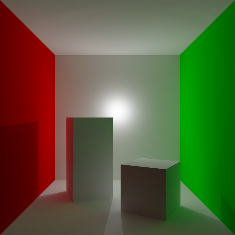
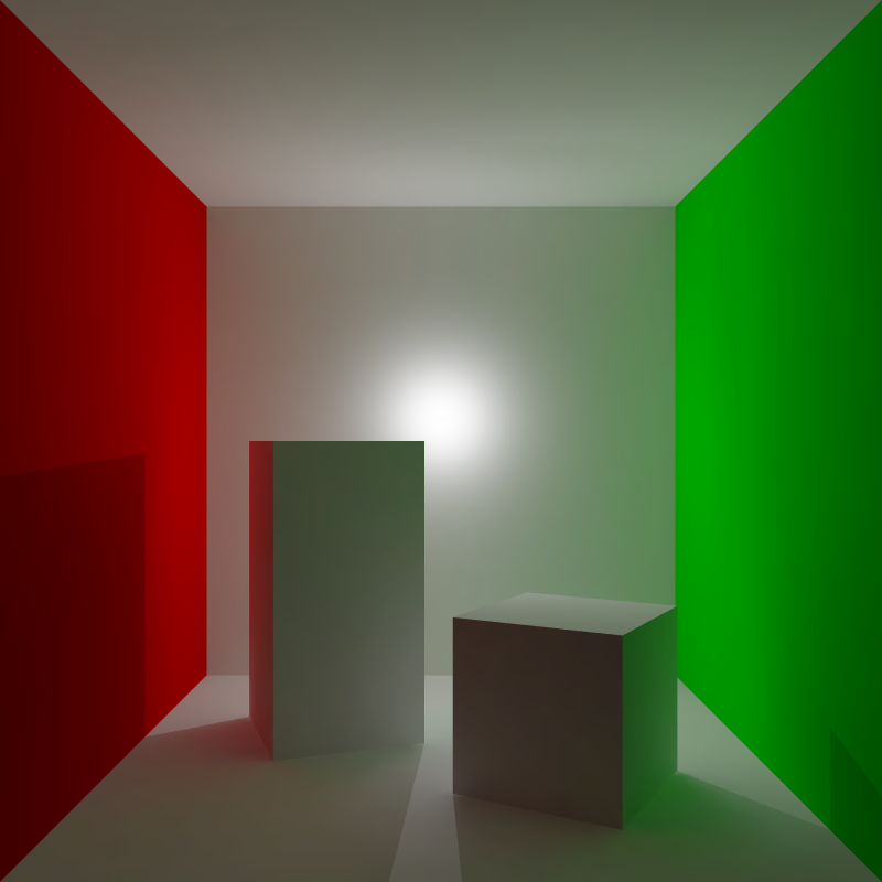
In the last post, I explained the basics of the global illumination algorithm I have been experimenting with. I was deliberately brief when discussing the calculation and compression of form factors because I was planning to devote an entire post to the subject (this one). We continue with the simple test scene from the last post to keep some continuity (depicted in Figure 1).
Ray tracing form factors
To recap, a form factor is a scalar that decides how much irradiance is exchanged between two texels in the light map. It can be calculated as the normalized solid angle one texel occupies as seen from the hemisphere at every point on the surface of the other texel, combined with a geometric factor. Without dwelling on the mathematical details, it's sufficient to say that we can sample this double integral using ray tracing. We take care of the geometric factor by sending rays with cosine weighted importance sampling. This is rather well known and instead of explaining the math I'll just include a code snippet at the end of this post on how to generate cosine weighted ray directions around a normal (the normal of the texel we are sampling from). The result is that each ray hitting a texel results in a form factor with value 1 over the number of samples taken. Multiple hits to the same texel simply add to the form factor value for that texel.
For each texel, in texture space, we must determine where in 3D space to sample. In my implementation, I determine potentially overlapping triangles in texture space by conservatively rasterizing the triangles in 2D using the texture coordinates. The result is a list of potentially overlapping triangles for each texel. The next step is clipping the overlapping triangles against the four sides of the texel, while retaining the 3D position of each vertex of the resulting polygons. A fixed number of samples are then distributed across the polygons, based on their respective surface area. I'm currently generating samples over the surfaces and ray directions using correlated multi-jittered sampling.
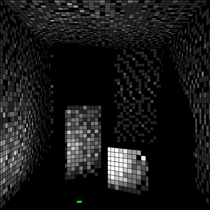
So now we simply send a few thousand rays per texel and get great results? Unfortunately that is not really the case as is apparent in Figure 2. If we ever hope to efficiently compress the form factors we need to get rid of this noise. We can always crank up the sample count, but at great expense. The better option is arguably to do some filtering.
Noise and sample density
The root cause of noise is insufficient sample density. The first step in fixing that is to estimate the sample density at a hit. Because all rays originate from approximately the same region in 3D space, sample density mostly varies with the angle from the texel normal (because of the cosine weighted random direction). I derived an expression for the filter size, which can be found at the end of the post in an appendix.
The filter radius is transformed into texture space of the surface that is hit, similar to how it's done for ray differentials. To transform a world space filter into texture space, I use the same formulation with 3 planes as the ray differentials paper. The difference is that instead of differential vectors, I have a single scalar. Using the planes I determine the maximum rate of change for each triangle, resulting in a single scalar that maps a world space filter radius to a texture space filter radius, as

where P are the planes and u/v are coordinates in texture space for each vertex. To get from the initial filter radius to a world space filter radius at a hit, I first propagate the filter radius by multiplying it with the distance to the hit. I then project it to the plane of the surface. Ray differentials are projected by dividing with the dot product between the ray direction and the surface normal. This doesn't really work for a radius. The radius is proportional to the square root of sample density and sample density should be scaled with the aforementioned dot product. The radius should therefore be divided by the square root of the dot product. I also added a maximum filter scale based on relative orientation to avoid large filters that stretch behind the texel we are sampling from, which can cause light bleeding (the boxes against the floor). The final filter propagation can be expressed as

where t is the distance along the ray to the hit surface, d is the ray direction, nh is the hit surface normal, nt is the texel normal, and r is the initial radius from the estimate described in appendix. This new filter radius can then be used to filter light map texels.
Before filtering, the maximum number of form factors to consider equals the sample count. Filtering naively could result in an explosion in the number of nonzero form factors to consider. I avoid this problem by filtering and compressing at the same time. To explain how, I first need to introduce the concept of an hierarchical light map.
Hierarchical light map
In order to efficiently filter, compress, and evaluate form factors, a multi-resolution representation of the light map is needed. One intuition is that as sample count is increased (approaching ground truth) texels far away contribute less and less. Then it makes sense to combine texels into larger patches, which also reduces the need to sample excessively to achieve an appropriate sample density. The solution I chose is quite simple. I create a mip map hierarchy over the light map texels. This provides multiple benefits:
- At precompute time, samples can be filtered by inserting them at the appropriate level in the pyramid.
- At precompute time, lossy compression can be performed by replacing individual form factors with their average contribution in a higher mip level.
- At runtime, input illumination can be prefiltered into a mip hierarchy so that form factors for multiple texels can be evaluated simultaneously.
- At runtime, direct illumination can be injected into the appropriate mip level, thus avoiding aliasing issues from using a low resolution cube map.
One detail is that if filtering is performed directly on irradiance, small texels may contribute too much in a higher mip level. It is therefore important that filtering is performed on radiance and not irradiance, i.e., the surface area contained within a texel need to be considered during filtering.
In order to avoid light bleeding between different geometrical features, a separate light map hierarchy is built for each island in texture space.
Filtering and compression


As I already mentioned, filtering amounts to inserting samples at some level in the mip map hierarchy. The appropriate mip level is selected using the filter radius that is computed for each sample. Because there's a separate hierarchy per island in texture space, I first determine which island each sample falls into, and then proceed to process each island in turn. I found that it's important to allow form factors in overlapping levels in the hierarchy, in order to avoid visual discontinuities as form factors jump from one level to the other.
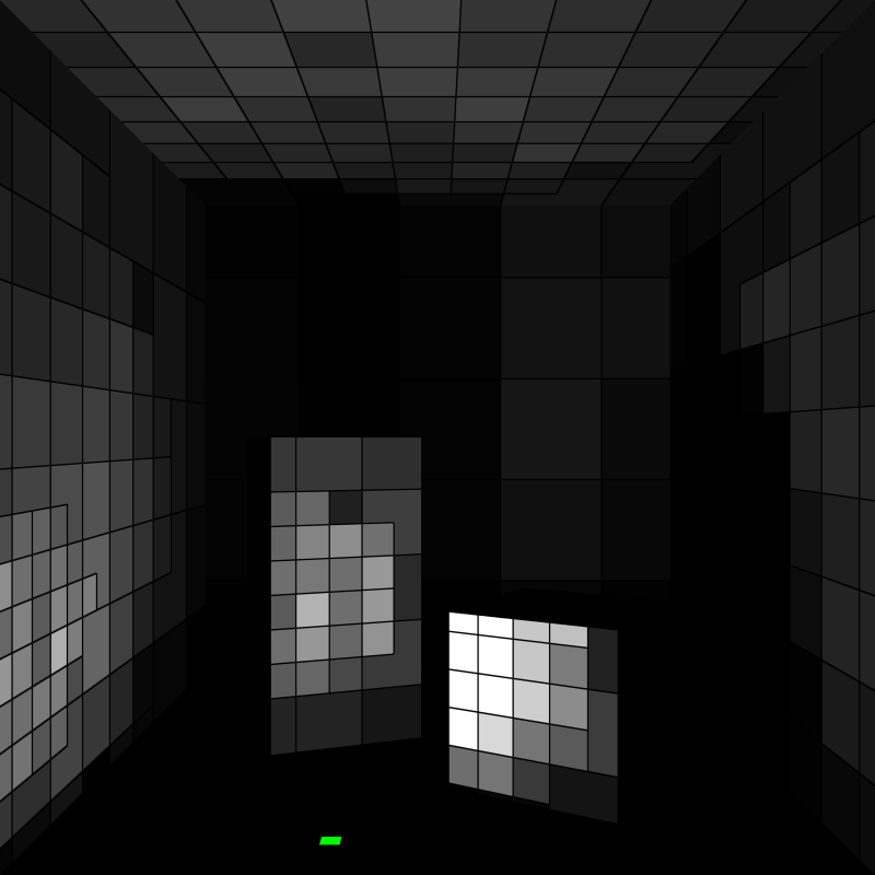
Both filtering and compression are controlled using the density parameter that is specified when calculating the filter radius. The result of filtering and compressing with a few densities can be seen in Figure 3. While the differences are quite small, the 0.01 density looks best in my opinion, even when compared to no compression (Figure 1) because it has less noise. Note that even the 0.1 version retains detail near objects, because of the adaptiveness of the filter radius calculation.
More improvements?
There are definitely some low hanging fruits for improving things further, but I think doing them would only complicate the post at this point. Instead I'll just mention some ideas here.
It's very likely that more can be done to improve the compression ratio. After filtering, it's certainly possible that some neighboring form factors on the same level in the hierarchy have similar weights. In that case it would make sense to merge them. Similarly, if a low resolution form factor is completely covered by higher resolution versions, the lower frequency information could be combined with them. Finding similarity in entire sets of form factors between neighboring texels and only encoding a delta seems like a promising idea too. Note that all these improvements would speed up the runtime computations as well, because of fewer form factors to evaluate per texel.
Regarding the quality of the light map, samples are currently inserted into the nearest texel and the nearest mip level. It may be possible to improve the approximation from large texels by inserting one sample into four neighboring texels (with appropriate weights), essentially performing bilinear filtering across texels. Or alternatively, to keep the contribution to a single form factor, russian roulette could be used to select between the neighbors. The same idea could also be extended to interpolate between levels in the hierarchy. Finally, something as simple as a more carefully laid out light map, without partial texels along the edges, could probably improve things a lot.
I'll likely try all these ideas at some point, but the results I'm getting seem good enough for now. In the next post I'm planning to address scalability and modularization.
Appendix: Estimating sample density
My first attempt was to use ray differentials. The cosine weighted ray direction is given by

where x and y are uniform random numbers (compare to cosine_weighted_direction). Differentiating gives:

Unfortunately, I found the result to be hard to control since the expression goes to infinity as the ray approaches the texel plane, with no obvious fix. Any filter radius estimate I derived from these expressions tended to either overestimate or underestimate the real sample density in some places.
My second attempt was to calculate the sample density over the hemisphere within an angle, a, of the ray direction. This results in the following integral:

Here, dz is the local z-coordinate of the direction vector. (It can also be computed by taking the dot product between the texel normal and the world space direction.) These expressions can be used to directly solve for a filter radius, r, for a planar surface at unit distance given a desired sample density:

While this removed the problem of estimating a filter radius, the expression still contains a singularity. This time, however, there's a simple geometrical interpretation. The cosine factor goes negative at the horizon of the hemisphere (which is incorrect). We can fix that by only considering positive values:

The downside is that we lose the closed-form expression. One option is to construct a lookup table from this integral but I instead opted to find an approximate expression. Let's find where the filter region just touches the border, which is the point where the error starts:

I then simply cap the radius to that value:

I also tried a more complicated approximation that found the correct value at the horizon (this value can interestingly be calculated with the solution to Kepler's equation), but it didn't seem worth it. For example, a large filter radius near the horizon can cause light bleeding, which may be worse than noise.
Appendix: Cosine weighted ray direction
Pseudo code for generating a cosine weighted random direction around a normal, given the normal and two uniform random numbers between 0 and 1.
vec3 u = tangent(n);
vec3 v = cross(n, u);
return (u*cos(a) + v*sin(a))*sqrt(y) + n*sqrt(1-y);
return normalize(t);
Go to part 3.